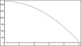
| Here’s another guest post from Allison Taylor at Wolfram Research. Today we’re looking at how to build simple physics models using the Wolfram Language If you’ve taken any introductory physics course, you’ve learned about Newtonian mechanics—conservation of energy and momentum, friction, harmonic motion, and so on. Idealized, classical motion can be broken down into a series of simple equations based on position, acceleration, and velocity. To derive these equations requires solving differential equations—something the Wolfram Language does very well with a function called NDSolve[]. For example, to model basic freefall, we just need to determine our initial conditions—acceleration y” is given by gravity, 9.81 m/s²; initial position is 150 m; and initial velocity y’ is 0. From these conditions, NDSolve[] can figure out the motion for a given range.
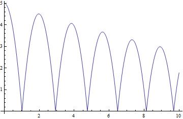
produces: So, in the above case, if I dropped a ball from a height of 150m, it would take approximately 5 seconds to reach the ground. Simple! But we can take this a step further with a function called WhenEvent[]. If I were to try to model a bouncing ball by hand, for example, I’d have to reevaluate the equations of motion every time the ball reached an “event” or change in conditions. The ball is in freefall from the air to the ground—but I can’t rely on those same values to model the ball bouncing from the ground back into the air. Using WhenEvent[] inside NDSolve[] lets you specify what happens when y[t]=0, or when the ball hits the ground. For this example, let’s say that when the ball hits the ground, it will reverse direction at 95% of its original speed. Now, every time the ball hits the ground, its velocity magnitude will continue to decrease by 5%. All inside one NDSolve[]—no more additional work for us!
produces: Having these values automatically computed means we can also easily observe how energy changes over time. Take the values of position and velocity that are calculated and plug them into the classical equations for kinetic and potential energy:
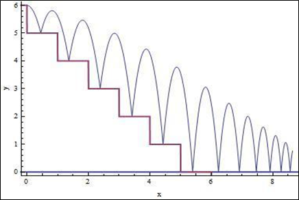
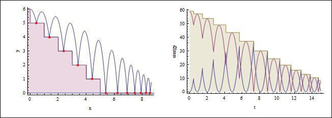
produces: The graph on the left shows the ball’s position, and the graph on the right shows the potential energy in red, kinetic energy in blue, and total energy in brown. Notice that the total energy decreases stepwise with each energy-dissipating bounce. And further! What if the ball was not bouncing on even ground? What if, instead, the ball was bouncing down a flight of stairs? The same principles are used, with an additional a[t] specifying how many steps of width one the ball must drop down. When the ball reaches the end of the stairs, “RemoveEvent” is used to stop the condition from continuing to be in effect.
produces: And again, we can also model the energy alongside it, and have the Wolfram Language punch up the graphics using Reap[] and Sow[] to obtain the coordinates of the ball at each bounce.
produces: Event[] inside NDSolve[] can be used to model all sorts of processes—from friction models to signal processing, to even simulating the human heartbeat. It lets you visualize many complex environments in a simple, cohesive way. Try it out! |
A Semi-automated Technology Roundup Provided by Linebaugh Public Library IT Staff | techblog.linebaugh.org
Wednesday, February 5, 2014
Modeling Physics with the Wolfram Language
Subscribe to:
Post Comments (Atom)


No comments:
Post a Comment